Introduction to R
The material below briefly describes the history of R and some of its core functions/data structures. Information on this webpage was sourced from a number of areas (as I have come to learn R over the past couple years), including R documentation, Advanced R, R for Data Science, and many other references and content found on the internet. Note that this text is not comprehensive or complete. Consult the official R documentation and other references for a more thorough coverage of R. All mistakes are my own.
History
The R project started off as a small endeavor by Ross Ihaka and Robert Gentleman at the University of Auckland in the early 1990s and found its way to a stable beta version by 2000. The syntax and interactivity of R was modeled after the S programming language. Martin Mächler of ETH Zurich convinced the two creators to make R's source code available as free software. This official happened in June 1995 when the creators released the source code under the terms of the Free Software Foundation's GNU general license. To learn more about the history of R see here and Wikipedia.
What is R?
R is a statistical computing language primary used for data analysis. While some may be wary of using the language (those who consider themselves not programmers), R is interpretted and easy to use. In other words, a full program does not have to be compiled to get things done. The syntax is intuitive, terse, and interactive. In just a one line of code, you can define a linear regression model:
lm(mpg ~ hp, data = mtcars)And in another couple lines of code, we can fit several linear models and store them in a data frame:
library(tidyverse)

mtcars %>%
  group_by(cyl) %>%
  nest() %>%
  mutate(model = map(data, ~ lm(mpg ~ hp, data = .x)))
#>     cyl data             model
#>     dbl list             list
#> 1     6 tibble [7 × 10]  S3: lm
#> 2     4 tibble [11 × 10] S3: lm
#> 3     8 tibble [14 × 10] S3: lm
The code above employs a decent amount of magic to abstract away details someone performing data analysis are not concerned with typically. For example, map() handles the construction of a for loop, which performs a function – in this case lm() – on each of the nested data frames. nest() respects the group_by() call creates a list column within the data frame. To say the least, this data frame is a rich object which includes a list of grouped data and list of linear models.
One last important detail to note here is the use of library(tidyverse). library() loads a library that is not included in base R into the environment. These libraries are typically downloaded from repositories, with the most popular being CRAN, the Comprehensive R Archive Network. Base R comes with hundreds of useful and important functions for statistical analysis and data mining; however, in order for R to maintain stability, new features (breaking changes) have not been added in quite some time. As a result, innovation and creativity happens outside of the core base R source code.
In the example above, we used the tidyverse consortium of packages to employ functions like group_by(), nest(), mutate(), and map(). We will end this note here and focus the rest of the documentation on the fundamentals of R.
Data Types
R has a variety of data types:
- Vectors
- Lists
- Matrices
- Arrays
- Data Frames
Vectors
Vectors are the least complex of all the objects above. Note that in R there are no scalars; everything is a vector. A scalar is represened as a vector of length one. Vectors are atomic, meaning they can only hold one data type. There are many vector types vectors can hold, including the following:
| Data Type | Example |
|---|---|
| Logical | TRUE, FALSE |
| Numeric | 32.3, 5, 767 |
| Integer | 5L, 2L, 20L |
| Complex | 2 + 6i |
| Character | "apple", "FALSE", "1" |
| Raw | "Hello World" is stored as 48 65 6c 6c 6f 20 57 6f 72 6c 64 |
In addition to the data types above, there are augmented vectors which enhance a certain data type to represent more abstract information. The two most common augment vectors are factors and dates. Factors are enhanced integer vectors and dates are enhanced double vectors.
nature <- factor("tree")
class(nature)
#> [1] "factor"

attributes(nature)
#> $levels
#> [1] "tree"
#>
#> $class
#> [1] "factor"

typeof(nature)
#> [1] "integer"

new_year <- as.Date("2019-01-01")
class(new_year)
#> [1] "Date"

attributes(new_year)
#> $class
#> [1] "Date"

typeof(new_year)
#> [1] "double"
You can access the content of a vector with
[[ operation.
fruits <- c("apples", "oranges", "berries")
fruits[[1]]
#> [1] "apples"
fruits[[2]]
#> [1] "oranges"
Lists
Lists are more complex than vectors and can hold many data types and objects. The example in the Introduction demonstrated the power of lists holding data frames and model objects.
new_list <- list(1, 2, 3)
print(new_list)
#> [[1]]
#> [1] 1
#>
#> [[2]]
#> [1] 2
#>
#> [[3]]
#> [1] 3
You can access elements of a list with $ [ and [[.
$ works on named lists.
new_list <- list(one = 1, two = 2, three = 3)
new_list$one
#> [1] 1
[ performs top-level extraction returns a list of the subset specified. [[ combined with [ with extract the elements of the list specified by [.
new_list[1]
$one
#> [1] 1

new_list[1][[1]]
#> [1] 1

list(1)
#> [[1]]
#> [1] 1
Matrices
A matrix is a two-dimensional rectangular data set. A vector can used as an input to the matrix function, along with the dimensions specified.
fruits <- c("apples", "oranges", "berries", "mangos")
matrix(fruits, nrow = 2, ncol = 2)
#>         [,1]      [,2]
#> [1,] "apples"  "berries"
#> [2,] "oranges" "mangos"
Arrays
An Array is similar to a matrix with the flexibility of having more than two dimensions.
veggies <- c("carrots", "lettuce")
array(veggies, dim = c(2, 3, 2))
#> , , 1
#>
#>         [,1]      [,2]      [,3]
#> [1,] "carrots" "carrots" "carrots"
#> [2,] "lettuce" "lettuce" "lettuce"
#>
#> , , 2
#>
#>         [,1]      [,2]      [,3]
#> [1,] "carrots" "carrots" "carrots"
#> [2,] "lettuce" "lettuce" "lettuce"
Data Frames
Data frames are tabular objects in R. They are used commonly to store data for the purposes of data analysis. A data frame can be created with the data.frame() function with vectors supplied to each named argument. If the vectors are named, then the names will represent each column. Note that each column of a data frame must be the same length and the type for each row must be the same with respect to the columns.
food <- data.frame(fruits, veggies)
food
#>     fruits veggies
#> 1  apples carrots
#> 2 oranges lettuce
#> 3 berries    kale
#> 4  mangos    kale
Functions
John Chambers, the creator of the S programming language and major contributor to R stated the following:
To understand computations in R, two slogans are helpful.
- Everything that exists is an object.
- Everything that happens is a function call.
– John Chambers
This quote is rich in meaning and has the depth to explained in a thorough text, but this stackoverflow answer is pretty good. In essence, everything in R is an object. Objects in R are data (even arguments of objects are objects), which can be manipulated at will prior to evaluation. One important note on how objects are modified: R has a particular way of modifying objects, referred to as copy-on-modify. In essence, if more than one name is binded to an object in R, a copy is made and the original object is not modified. If only one name is binded to an object, R will copy-in-place. This is covered in detail in Advanced R and R's official documentation, so I will end this discussion here.
saved_call <- quote(mtcars %>%
                    group_by(cyl) %>%
                    nest() %>%
                    mutate(model = map(data, ~ lm(mpg ~ hp, data = .x))))
saved_call
#> mtcars %>% group_by(cyl) %>% nest() %>% mutate(model = map(data, ~lm(mpg ~ hp, data = .x)))

saved_call[[2]] <- substitute(mtcars %>% group_by(gear) %>% nest())
saved_call
#> mtcars %>% group_by(gear) %>% nest() %>% mutate(model = map(data, ~lm(mpg ~ hp, data = .x)))

eval(saved_call)
#> A tibble: 3 x 3
#>    gear data               model
#>     dbl list               list
#> 1     4 tibble [12 × 10] S3: lm
#> 2     3 tibble [15 × 10] S3: lm
#> 3     5 tibble [5 × 10]  S3: lm
In the above example, we changed the original coded used in the Introduction to reflect a different group_by(). We then evaluated the new call and received a different object than the original. This leads to the second slogan: the evaluation of objects almost always happens due to a function call. Even subsetting operations are functions.
class(`[[`)
#> [1] "function"
class(`$`)
#> [1] "function"
class(`+`)
#> [1] "function"
R even allows you to modify operands, something other programming languages typically do not allow.
`+` <- function(x, y) sum(x, y) * 1000
1 + 1
#> [1] 2000
This allows for powerful creativity, such as the case with ggplot2, a graphics library used for plotting in R. ggplot2 uses `+` to modify/add objects to the original ggplot call.
ggplot(mtcars, aes(mpg, hp)) +
  geom_point() +
  labs(title = "HP vs. MPG")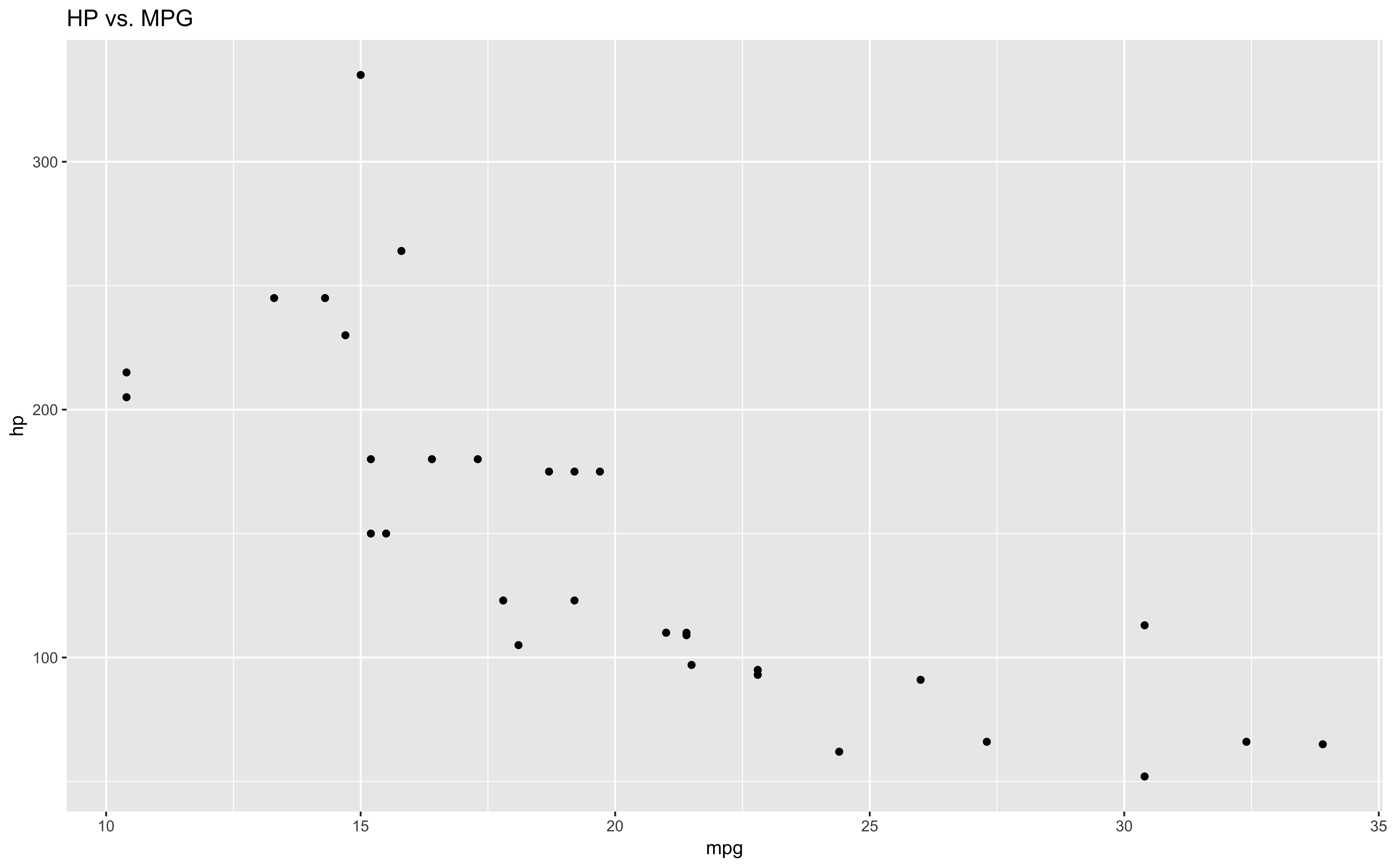
Basics
We have discussed some deep concepts with functions in R. To back up a bit, let's discuss some basics and practical implementations. Functions typically have arguments, which modify the object the function is called on in different ways (remember arguments are objects also). Let's create a simple function with one argument that does not exist in base R.
prime <- function(x) !(x %% 2 == 0)
prime(5)
#> [1] TRUE
prime(2)
#> [1] FALSE
But what happens if a user inputs a non-numeric argument?
prime("apples")
Error in x%%2 : non-numeric argument to binary operator
This return is fine and intuitive. You have to pass a number to a function that checks if a number is prime. However, what happens when a vector greater than length one is passed as an argument?
prime(5:10)[1]
#> TRUE FALSE  TRUE FALSE  TRUE FALSE
Since everything in R is a vector, it recycles through one argument to match the length of the vector provided. If the argument is not a multiple of the vector provided, a warning will be thrown. If we want to discard this behavior altogether, we can explicitly check for the length before execution.
prime <- function(x) {
if (length(x) > 1) {
    stop("x must be vector of length one.")
}

!(x %% 2 == 0)
}
References
Documentation and text was based in CRAN, R for Data Science, and Wikipedia.